The Geometry of Biological Memory: Why DNA Is Not the Only Blueprint
How to calculate a flatworm’s decision to grow two heads as a mathematical movement in a Bures-Wasserstein landscape.

When we think about the “memory” of biological forms, we almost inevitably think of DNA. DNA, according to the popular dogma, is the ultimate blueprint. It dictates where the head sits, where the tail grows, and how the tissue in between is supposed to look.
But what happens when this dogma cracks?
Take the planarian (a type of flatworm). If you cut off its head, a new one grows back. That is fascinating, but genetically explainable. However, researchers—most notably Michael Levin and his team at Tufts University—have achieved something truly mind-bending in recent years: if you briefly disrupt the worm’s bioelectric network with a chemical agent and then cut it, it suddenly grows two heads.
The truly crazy part happens months later: if you cut this two-headed worm in half again—this time without any chemical manipulation—the fragments will again grow into two-headed worms.
The worm’s DNA has not changed. It is absolutely identical to that of the single-headed wild type. Nevertheless, the tissue has “learned” and remembered that its new morphological goal (its target state) is now two-headed.
Form memory, therefore, does not reside exclusively in the genes, but in the physiological and electrical architecture of the tissue. The problem is: How do we capture this non-genomic memory mathematically? Purely gene-centric models fail here. Other approaches retreat into vague metaphors about “collective intelligence.” What we actually need is a formal, calculable kinematics.
This is exactly what I propose in my new preprint: Covariance Geometry of Bioelectric Pattern Memory: Bures-Wasserstein Target-State Transitions in Morphogenesis.
Where Exactly Does This “Memory” Live? The Secret of Covariance
To understand how a tissue can remember a shape, we have to ask how a network of cells can store information in the first place.
The answer does not lie in the isolated electrical voltage of a single cell, but in how the cells fluctuate together. When cells at the anterior and posterior ends of the worm communicate electrically, their signals are correlated.
This is where the math comes in: the tool used to measure such joint fluctuations and correlations in a network is called a covariance matrix (\Sigma). We can view the state of the tissue as a structured “cloud” of bioelectric correlations. The blueprint for “two-headedness” is permanently stored in the geometric shape of this cloud.
The First Amputation: How the Blueprint Changes
To understand why the tissue doesn’t forget, we have to look at what happens during that very first experiment.
In a healthy wild-type worm, the bioelectric pattern is strictly asymmetric—the pattern says “head here, tail there” (in my mathematical model, this is a polarity of s = -1). When researchers chemically disrupt the worm’s ion channels, they force the bioelectric network into a radical reorganization.
In the language of mathematics, this disruption acts as a squeezing operator. It “squeezes” the original covariance structure, redistributing the variance and shifting the polarity into the positive range (s = +1). When the worm is cut for the first time, its tissue is already in this artificially reversed state. It evaluates its geometric distance to the possible blueprints and determines: “I am now much closer to the two-headed attractor than the one-headed one.” And so, two heads grow.
That alone is spectacular. But the true miracle of biology—and the proof of genuine, stable “memory”—reveals itself months later during the second cut.
The Second Cut: Why the Tissue Doesn’t Forget
What happens when we cut the now two-headed worm a second time, long after the chemicals have washed away?
The amputation creates massive biological and electrical chaos (a nonspecific injury-induced variance, let’s call it \epsilon). If the memory were just a simple electrical “switch,” this chaos would instantly wipe the hard drive.
But because the memory is encoded in the deep covariance structure of the network, a residual fraction of this reprogrammed “fluctuation cloud” survives the cut. The tissue must now heal and restore a morphology. It faces a choice: which morphological target state (attractor) should it strive for—the one-headed or the two-headed blueprint?
Why Bures-Wasserstein? The Sandcastle Problem
At this point, mathematically speaking, the tissue rolls down a hill to minimize the error. But in what kind of space?
You might wonder: why don’t we just measure the distance to the target using a normal ruler (Euclidean distance)?
Imagine you have two sandcastles. One is here, the other is over there. If you measure the Euclidean distance, you simply draw a straight line between their peaks. For rigid, physical objects in space, this is perfect. But our biological memory is not a rigid object. It is a dynamic cloud of fluctuations. If you want to transform one cloud into another, a ruler doesn’t help. You need to know how much “sand” you have to shovel, and from where to where, to knead the shape of the first cloud into the shape of the second.
This is the core of Optimal Transport, which brings us to the Bures-Wasserstein (BW) metric.
The BW metric calculates the exact geometric “cost” of reshaping one distributed physiological pattern into another. This is crucial for biology: tissues must do physical work (opening ion channels, shifting gradients) to heal. While other geometric metrics merely measure the difference in information, the Bures-Wasserstein metric measures the work required to move mass and charge. Gradient descent in a Bures-Wasserstein landscape is the energetically and biophysically cheapest path to regeneration.
The Basin of Attraction
Because the tissue fragment still carries the residual, “squeezed” covariance polarity (s) of the two-headed worm despite the chaos of the injury, it is geometrically closer to the two-headed attractor in the Bures-Wasserstein space. It inevitably falls into the two-headed regenerative basin.
This is exactly what the mathematical model in my paper proves.
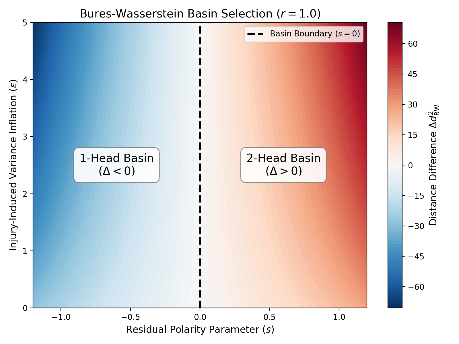
Phase diagram of the Bures-Wasserstein basin selection. The color gradient represents the difference in BW distance between the two target attractors.
As this phase diagram from the paper illustrates, covariance geometry delivers a strikingly clear, falsifiable result: the basin boundary runs strictly vertical at a neutral residual polarity of s=0.
This means: no matter how massive the noise and chaos of the amputation gets on the y-axis (the injury-induced variance \epsilon), it does not shift the decision boundary by a single millimeter. The tissue is not fooled by the sheer magnitude of the injury. The topological decision is dictated exclusively by the retained covariance polarity on the x-axis. The model mathematically separates the pure noise of an injury from genuine bioelectric structural memory.
Moving Beyond Metaphor
This framework operationalizes observations that have long been considered almost “magical” or, at the very least, hard to quantify. It provides a hard, geometric language for non-genomic pattern memory.
It shows that morphogenesis is not blindly executing a DNA code, but can be understood as a controlled gradient descent in a Bures-Wasserstein geometry, where macrostates communicate via their covariance. It takes the core biological axioms of Michael Levin’s TAME (Technological Approach to Mind Everywhere) framework and gives them a rigorous, calculable kinematics. We don’t need quantum mysticism to model complex, path-dependent tissue decisions. A rigorous covariance geometry, regularized by a biophysical “spectral floor,” is enough to formulate a testable theory of biological target states.
If you want to dive into the math—including the closed-form proofs of the covariance-squeezing distances in the appendix—you can read the full preprint on SSRN now:
👉 Read the paper here: Hamiltonian Lift of Bures–Wasserstein Covariance Dynamics with a Spectral Floor
What do you think? Is covariance geometry the right path to finally decoding the software of life? Let me know in the comments.